Kevin Park

Welcome to my data science portfolio. I am passionate about data analytics, data visualization, and machine learning that can provide insights and solve real-world problems.

Predictive models in category based on Carsales datasets

• This project is to build a tool to analyse, compare, predict and visualize the important features and price of different car categories or makes.
• Build such predictive models to facilitate decision making for second hand car buyers and sellers.
• Multiple Linear, Random Forest and Neural Network predictive modelling techniques were employed to create predictive models.
• The study implemented predictive models on actual data from Carsales website.
• Observe contributing features in category into different levels of prestige - luxury sports, luxury and economy cars.
• Drill down car categories to discover the price influencing features on different car makes.

Part 1. Dataset

A. Data extraction

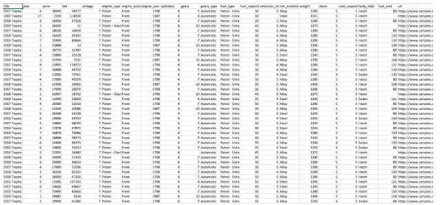
The sample dataset of Toyota Corolla extracted from Carsales website. Python’s Beautiful Soup v4 library used to extract data into a form that can be imported.

Following is an example of Toyota Corolla dataset in csv file extracted from Carsales website.

B. Data exploration

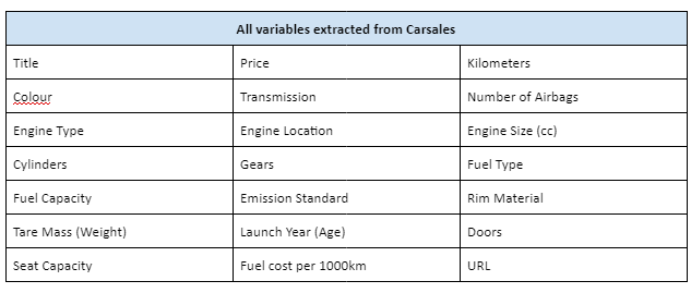
The dataset comprises of 21 attributes related to 2030 sold Toyota Corolla cars. The table has 2030 rows and 21 columns. Based on this dataset, the research needs to develop a reliable predictive model to predict the selling price of the cars. Therefore, the target variables applicable for model is ‘Price’.

As we have identified price as the target variable, the research has examined the prices of the Toyota Corolla vehicles by calculating the summary statistic and prepared the histogram, density and box plot of the price variable in the Toyota Corolla dataset. The price is a continuous numerical variable. The following are results of summary statistics and plots created in Python.

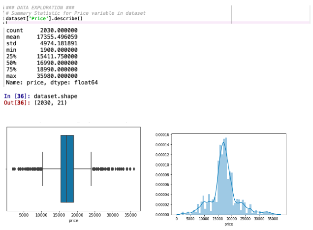
The summary statistic shows that, the selling price for Toyota Corolla has an average value of $16,990, standard deviation of $4,974 and mean of $17,355 (minimum from $1,900 to maximum $35,980) There is also indication of extreme values, which is shown in the histogram, density and boxplot.

C. Check for missing values

We need to check for any missing values in the Toyota Corolla dataset provided using isnull() function. Consequently, the plot below shows that, the dataset is free from any missing values.

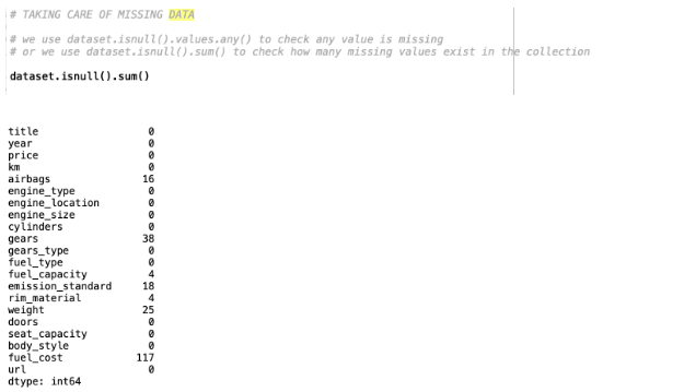
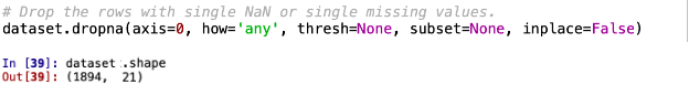
Having missing values in a dataset can cause errors with predictive modelling algorithms. The simplest strategy for handling missing data is to remove records that contain a missing value. We can use dropna() to remove all rows with missing data. The table has been cut from 2030 in the original dataset to 1894 with all rows containing a NaN removed.

D. Transformation of categorical values into numerical values

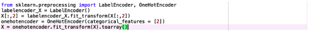
As regression models only take on numerical variable, it is important that we need to transform categorical variables into numeric variables to feed into the regression model. In this case, Fuel_Type variable identified as a categorical variable with two possible values which are Petrol and Diesel.

For transformation purpose, we assigned binary value in which 1 and 0 implies the car has the particular fuel type. The following Python script for transformation process shown below.

E. Correlations evaluation and dimensionality reduction

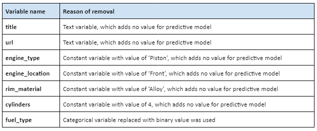
Following section shown the correlations between variables and carried out dimensionality reductions by removing several variables. Prior to evaluating the correlation, five variables were removed from the dataset. The table belows lists 5 variables removed and reasons for it.

The correlation plot below is prepared using the heatmap function after the first phase of removal.

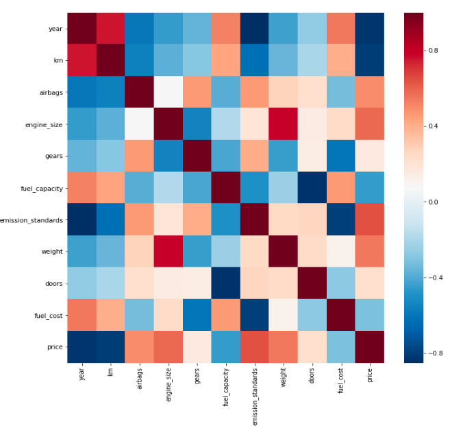
Following the correlation between variables shown above, dimensionality reduction is performed by removing high cross-correlation variables. Followed with a merge of target variable ‘Price’. It is also noted year, km, fuel_cost variables have high-correlation, which shows that they are important variables which later will be used in predictive modelling. Variable year, km have negative relationship with the sale price, which implies that older cars and long km are cheaper. Variable weight, emission_standards, engine_size and airbags implying increase the weight of the car has a positive effect on the sale price. Moreover, another features like fuel_capacity and fuel_cost have positive linear relationship implying includes these features have positive effect on the sale price.

Part 2. Regression Technique using Multiple linear regression

a. Regression models

In this section, multiple linear regression as a technique is applied for predictive modelling of the case study on Toyota Corolla dataset. As the main task for the predictive modelling is to predict the selling price of used Toyota Corolla using the variables selected in Part 1, therefore, price variable will be used as target variable.

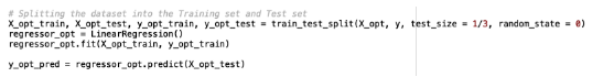
Prior to building the linear regression models, the dataset was partitioned with ⅔ as the training data sample and ⅓ as the testing data. The trained dataset comprises of 1262 training data and 632 testing data.

This is the process of building a model used backward elimination.

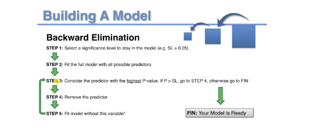
From step 1, select a significance level to stay in the model, for example, SL = 0.05 applied in this method. Step 2, fit the full model with all possible predictors. After you fit the model, you will see the one with the highest p-value, so if the p-value is greater than the significance level then you go to step 4. Step 4 is to remove that predictor. It is to remove basically the variable that has the highest p-value. And step 5, you fit the model without this variable. The model will be rebuilt with the fewer number of variables. In step 5, continue to fit the model again with one less variable. This process will keep doing that until it comes to a point where the variable of that p-value is still less than the significance level, then go to FIN (means model is ready).

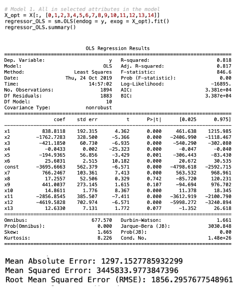
1) Regression Model 1.

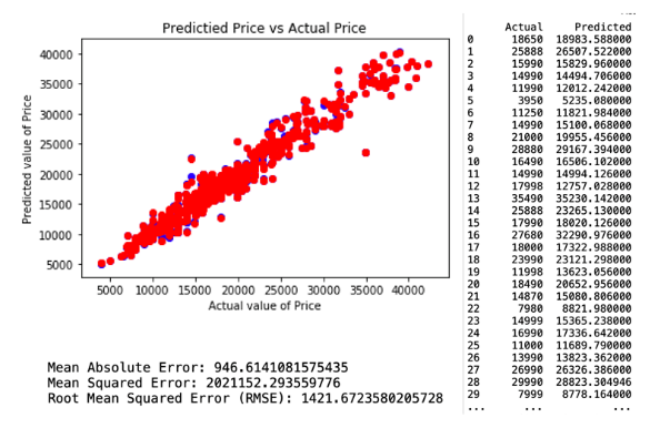
The first regression model technique predictive model has included all of the attributes in the selected variables identified previously section. This model resulted in an adjusted R-squared of 0.817 and Root Mean Square Error (RMSE) of 1856.29. The regression and model evaluation result is shown below.

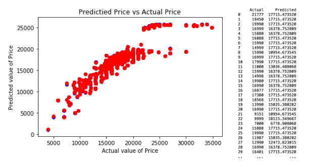
This is a comparison of predicted values with actual values and the scatter plot for regression model 1.

2) Regression Model 2.

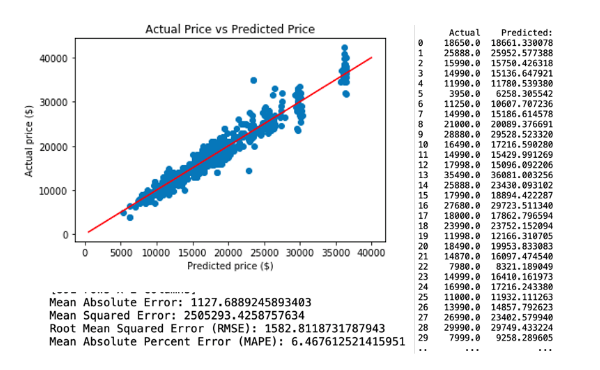
The attributes applied for regression model 2. comprises age, km, airbags, engine_size, gears, emission_standards, weight and fuel_cost. This model resulted in an adjusted R-squared of 0.817 and Root Mean Square Error (RMSE) of 1841.17. The regression and model evaluation result is shown below.

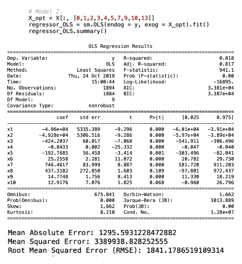
This is a comparison of predicted values with actual values and the scatter plot for regression model 2.

3) Regression Model 3.

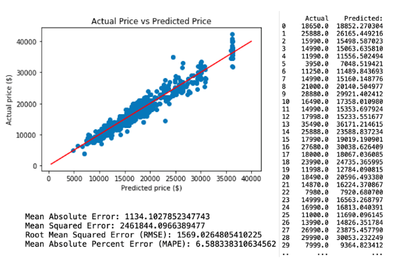
The attributes applied for regression model 3 comprises age, km and weight. This model resulted in an adjusted R-squared of 0.988 and Root Mean Square Error (RMSE) of 1957.55. The regression and model evaluation result is shown below.

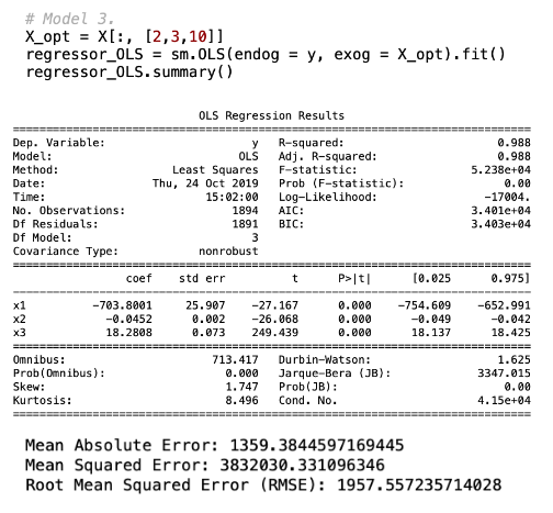
This is a comparison of predicted values with actual values and the scatter plot for regression model 3.

b. Evaluation

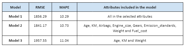
The table above summarises the results of three linear regression technique predictive models based on the Toyota Corolla dataset. RMSE is used to measure the difference between predicted variable and the actual variable. Therefore, the lower RMSE would be preferred, which implies that the model 2 is the most optimal linear regression predictive model.

Part 3. Regression Technique using Random Decision Tree

a. Regression models

In this section, random decision tree technique is applied for predictive modelling of Toyota Corolla dataset. This section summarises and evaluates four random decision tree predictive models to predict price.

Prior to building the random decision tree regression models, the dataset was partitioned with ⅔ as the training data sample and ⅓ as the testing data. The trained dataset comprises of 1262 training data and 632 testing data. Then, the number of trees in the forest of 1,000 is selected to fit a number of decision tree classifiers.

Decision trees makes split that maximize the decrease in impurity. By calculating the decrease in impurity for each feature across all trees we can know that feature importance. The Python script and figure of feature importance shown below.

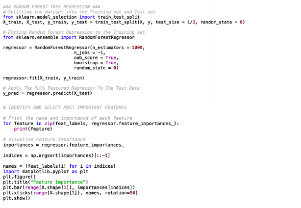
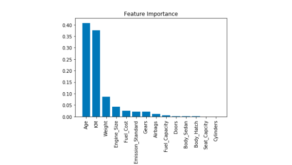
As can be seen from the graph, feature importance from Toyota Corolla shows that Age and KM are the highest features contributing to the final price followed by weight, engine size and fuel cost.

1) Regression Model 1.

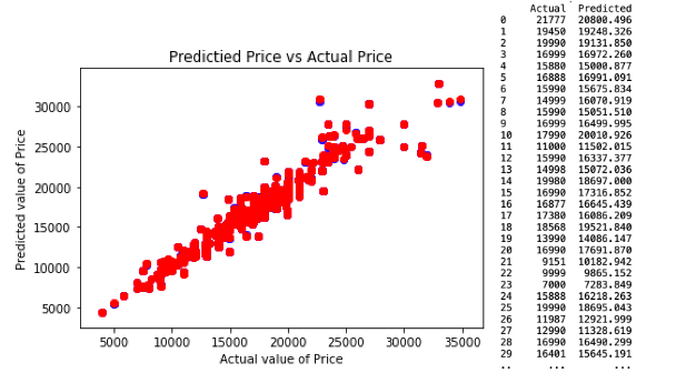
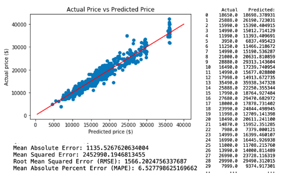
The first decision tree predictive model is created by applying all selected variables and resulted with RMSE of 1375.09. The python script and model evaluation result shown below.

This is a comparison of predicted values with actual values and the scatter plot for decision tree regression model 1.

2) Regression Model 2.

The second decision tree predictive model is created by applying features that have an importance of more than 0.01. There are 8 selected variables of feature importances, which comprises of age, km, airbags, engine_size, gears, emission_standards, weight and fuel_cost. This resulted with RMSE of 1383.16. The python script, feature importance and model evaluation result shown below.

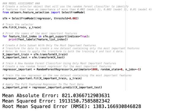
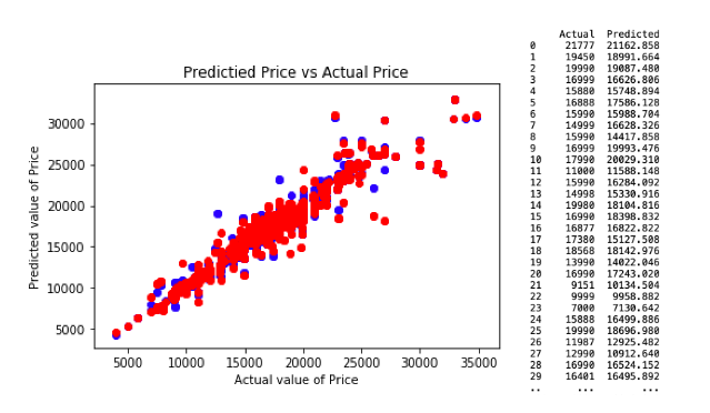
This is a comparison of predicted values with actual values and the scatter plot for decision tree regression model 2.

3) Regression Model 3.

The third decision tree predictive model is created by applying features that have an importance of more than 0.05. There are 3 selected variables of feature importances, which comprises of age, km and weight. This resulted with RMSE of 1581.61. The python script, feature importance and model evaluation result shown below.

This is a comparison of predicted values with actual values and the scatter plot for decision tree regression model 3.

This is a comparison of predicted values with actual values and the scatter plot for decision tree regression model 3.

b. Evaluation

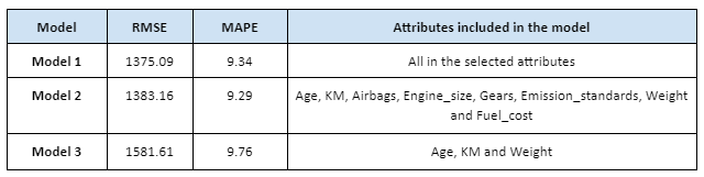
The table above summarises the results of four random decision tree predictive models, with price as the target variable. As explained in regression model evaluation, a lower RMSE is more preferred, which implies that the random decision regression model 1 is the most optimal decision tree regression predictive model. However, it is important to note that model 3 includes only age, km and weight, which may not be ideal for actual predictive model.

Part 4. Regression Technique using Neural Network

a. Regression models

In this section, neural network technique is applied for predictive modelling of Toyota Corolla dataset. The graph below shows what its looks like in neural network regression (can see some attributes as Inputs(Is) and one output layer which is the Price used Toyota Corollas) The Bs are biases introduced.

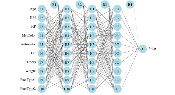
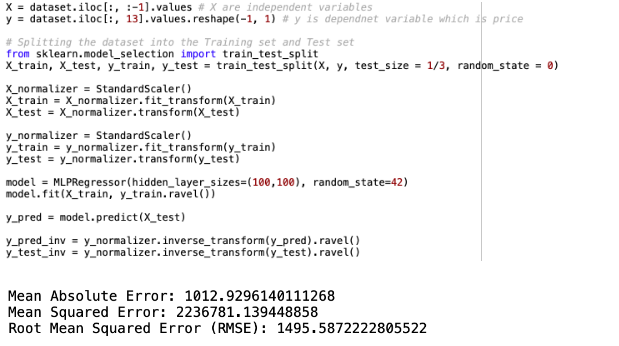
Prior to building the neural network regression models, the dataset was partitioned with ⅔ as the training data sample and ⅓ as the testing data. The trained dataset comprises of 1262 training data and 632 testing data. The model optimizes in multilayer perception layer, and the number of neurons (100, 100) applied in the hidden layer(Hs). Then a seed value of 42 used to generate random sampling dataset. Neural network is in general hard to see which input features are relevant and which are not. The reason for this is that each input feature has multiple coefficients that are linked to it - each corresponding to one node of the first hidden layer. Adding additional hidden layers makes it even more complicated to determine how big of an impact the input feature has on the final prediction. On the other hand, for linear models it is very straightforward since each feature has a corresponding coefficient and its magnitude directly determines how big of an impact it has in prediction. This research uses features selected from linear regression models (where reduced the number of features in model 1, 2 and 3) for neural network.

1) Regression Model 1.

The first neural network predictive model is created by applying all selected variables. This resulted with RMSE of 1495.58. The python script and model evaluation shown below.

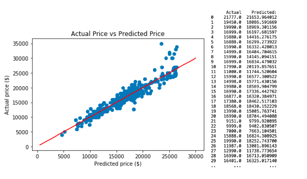
This is a comparison of predicted values with actual values and the scatter plot for neural network regression model 1.

2) Regression Model 2.

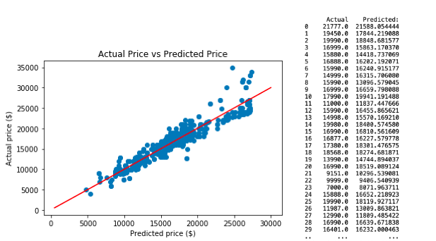
The second neural network predictive model is created by applying selected variables from random regression model 2, which comprises Age, Km, Airbags, Engine Size, Gears, Emission Standards, Weight and Fuel Cost. This resulted with RMSE of 1520.42. The python script and model evaluation shown below.

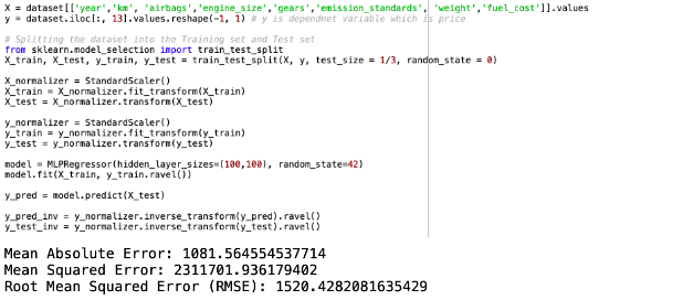
This is a comparison of predicted values with actual values and the scatter plot for neural network regression model 2.

3) Regression Model 3.

The third neural network predictive model is created by applying selected variables from linear regression model 3, which comprises Age, Km and Weight. This resulted with RMSE of 1548.81. The python script and model evaluation shown below.

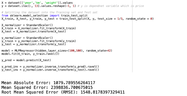
This is a comparison of predicted values with actual values and the scatter plot for neural network regression model 3.

b. Evaluation

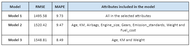
The table above summarises the results of four neural network predictive models, with price as the target variable. As explained in regression model evaluation, a lower RMSE is more preferred, which implies that the neural network regression model 1 is the most optimal neural network regression predictive model.

Part 5. Model comparison

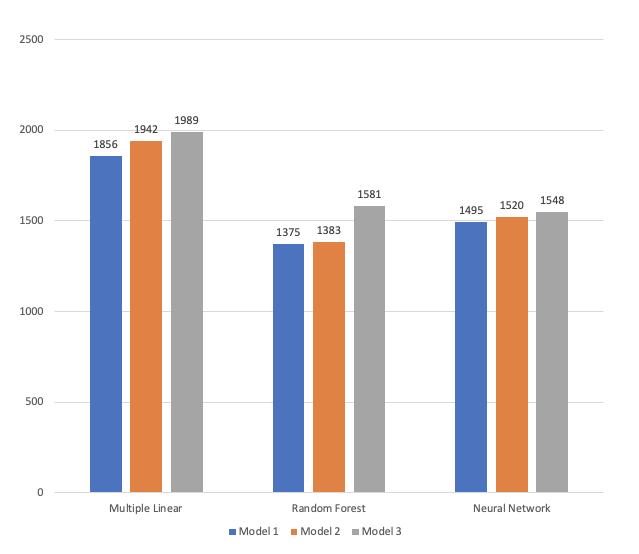
The graph above summarizes the results of three regression techniques (multiple linear/random decision tree/neural network) to predict car sales price from Toyota Corolla dataset. The accuracy of the predictive models are compared based on their RMSE. In terms of efficiency, the random forest and neural network regression technique is much more efficient compared to the multiple linear regression. From all of the above predictive models, the random forest regression technique model 1. has the lowest RMSE of 1375.09. The random decision tree algorithms also provide importance features and the relationships between the different variables, which helps to create more accurate models. One key highlights shows that 3 key features: Age, KM and Weight are the most importance features. Moreover, it appears that the results from random decision slightly outperformed the results from neural network models, by providing a more lower of RMSE. Consequently, the random forest tree technique model appears to be more suitable predictive modelling for the Toyota Corolla dataset from Carsales.

Part 2. Challenge: Categorizing the Used Cars

The car brand names and make for a vehicle tells a lot about the level of prestige of a car, for example, Mercedes-Benz and BMW are luxury car makers, which can be in the luxury segment. In this research, we will categorize and test on used car based on different in the level of prestige. The 3 categories are Luxury Sports, Luxury and Economy. The proposed categories and their respective makes are as follows:

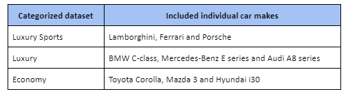
A. Luxury Sports

The dataset comprises of 21 attributes related to 790 Luxury Sports cars which contains 3 car makes (100 samples from Lamborghini, 109 from Ferrari and 581 from Porsche where extracted from Carsales site).

1. Multiple Linear Regression

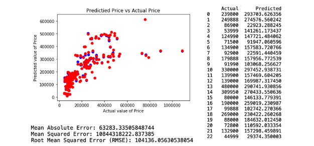
a. Regression Model 1.

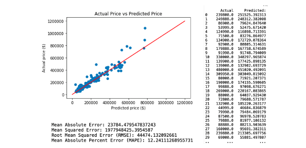
The first regression model technique predictive model has included all of the attributes in the selected variables identified previously section. This model resulted in a Root Mean Square Error (RMSE) of 104136.05. The regression and model evaluation result is shown below.

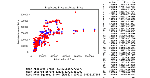
b. Regression Model 2.

The attributes applied for regression model 2. comprises Age, KM, Airbags, Engine Size, Cylinders, Gears, Fuel Capacity, Emission Standard, Weight, Doors, Seat Capacity and Fuel Cost. This model resulted in a Root Mean Square Error (RMSE) of 109712.18. The regression and model evaluation result is shown below.

c. Regression Model 3.

The attributes applied for regression model 3. comprises KM, Engine Size and Weight. This model resulted in a Root Mean Square Error (RMSE) of 117433.77. The regression and model evaluation result is shown below.

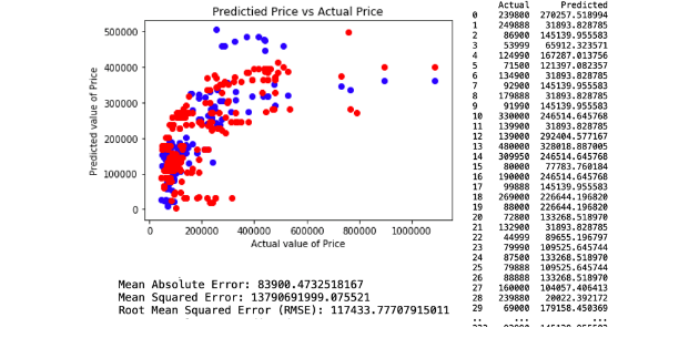
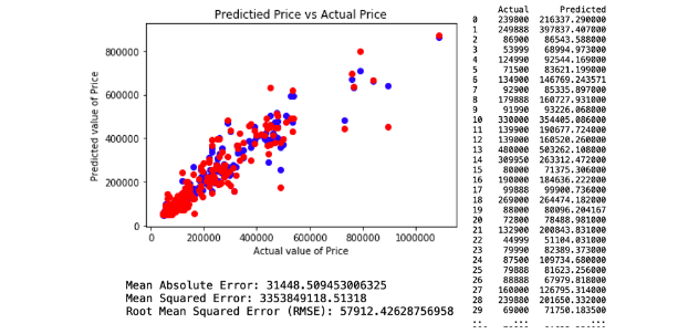
2. Random Forest Regression

As can be seen from the graph, feature Importance for Luxury Sports shows that KM and Engine Size are the highest features contributing to the final price followed by Weight, Doors and Fuel cost.

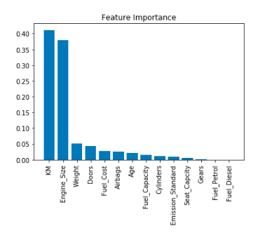
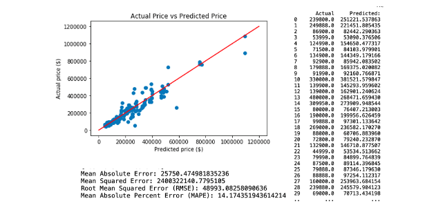
a. Regression Model 1.

The first decision tree predictive model is created by applying all selected variables and resulted with RMSE of 45260.87. The regression and model evaluation result is shown below.

b. Regression Model 2.

The second decision tree predictive model is created by applying features that have an importance of more than 0.01. There are 9 selected variables of feature importances, which comprises of Age, KM, Airbags, Engine Size, Cylinders, Fuel Capacity, Weight, Doors and Fuel Cost. This resulted with RMSE of 45771.93. The regression and model evaluation result is shown below.

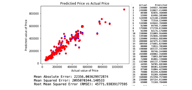
c. Regression Model 3.

The third decision tree predictive model is created by applying features that have an importance of more than 0.05. There are three selected variables of feature importances, which comprises of KM, Engine Size and Weight. This resulted with RMSE of 57912.42. The regression and model evaluation result is shown below.

3. Neural Network Regression

a. Regression Model 1.

The first neural network predictive model is created by applying all selected variables. This resulted with RMSE of 44474.13. The regression and model evaluation result is shown below.

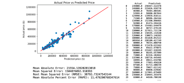
b. Regression Model 2.

The second neural network predictive model is created by applying selected variables from random tree regression model 2, which comprises Age, KM, Airbags, Engine Size, Cylinders, Fuel Capacity, Weight, Doors, Fuel Cost. This resulted with RMSE of 38792.73. The regression and model evaluation result is shown below.

c. Regression Model 3.

The third neural network predictive model is created by applying selected variables from random tree regression model 3, which comprises KM, Engine Size and Weight. The regression and model evaluation result is shown below.

4. Model Comparison

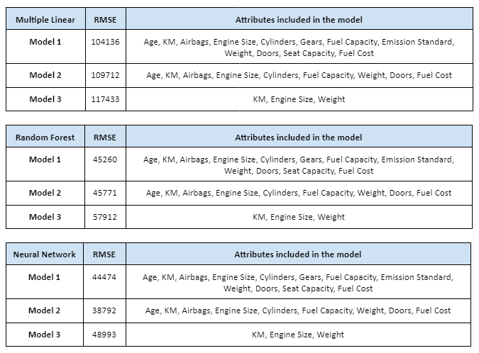
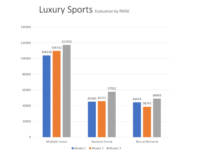
The graph above summarizes the results of three regression techniques (multiple linear/random decision tree/neural network) to predict car sales price from Luxury Sports dataset. The accuracy of the predictive models are compared based on their RMSE. In terms of efficiency, the random forest and neural network regression technique is much more efficient compared to the multiple linear regression. From all of the above predictive models, the neural network regression technique model 2. has the lowest RMSE of 38792. Random forest shows that KM and Engine Size are the most important features. Moreover, it appears that the results from neural network outperformed the results from random forest models, by providing a more lower of RMSE. Consequently, the neural network technique model appears to be more suitable predictive modelling for the Luxury Sports dataset from Carsales.

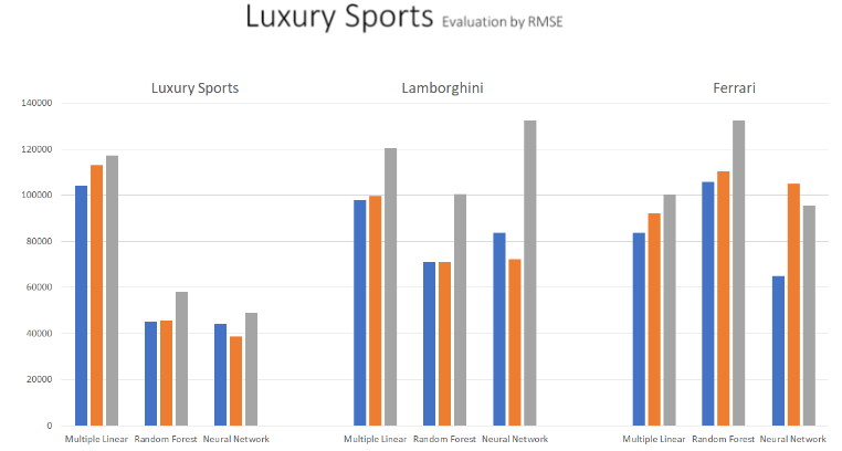
The graph above illustrates all results of three regression techniques (multiple linear/random decision tree/neural network) to predict car sales price from Luxury Sports, Lamborghini and Ferrari dataset. The accuracy of the predictive models are compared based on their RMSE. When we go deep into more specific car makes, for example, Lamborghini and Ferrari in Luxury Sports. As you see from Luxury Sports, neural network outperform multiple linear and random forest, however, random forest and neural network performs similar in Lamborghini dataset. From Ferrari dataset, it appears that the result from neural network Model 1. outperformed all results from multiple linear and random forest, by providing a much more lower of RMSE. However, all multiple linear regression models appears lower RMSE than Random Forest models in Ferrari Dataset. Overall, the neural network technique model appears to be more suitable predictive modeling for all Luxury Sports, Lamborghini and Ferrari cars.

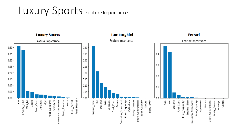
The charts above shows all the feature importance using Random Forest regression, compared with Luxury Sports, Lamborghini and Ferrari car makes. The luxury sports data shows that KM and Engine Size are the most influential features to predict car sales price. However, Lamborghini dataset appears that Engine Size is a significant factor contributing to the price more than KM. The weight and age of used cars are the next important characteristics in Lamborghini dataset. On the other hand, it appears that the most substantial features of used cars in Ferrari dataset are Age and KM, not Engine Size. As you can see, most of the Luxury Sports includes Lamborghini car makes, KM and Engine Size are the crucial features of used car sales, but not for Ferrari car makes. Overall, these charts shows that all Luxury Sports, Lamborghini and Ferrari have different car factors vital to the used car prices.

B. Luxury Cars

1. Multiple Linear Regression

The dataset comprises of 21 attributes related to 1809 Luxury cars which contains 3 car makes (1013 from BMW 3 series, 705 Mercedes-Benz E Class and 91 Audi A 8 series where extracted from Carsales website).

a. Regression Model 1.

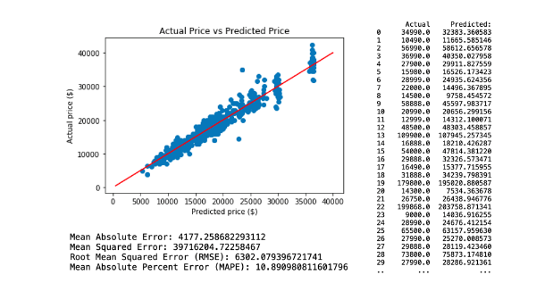
The first regression model technique predictive model has included all of the attributes in the selected variables identified previously. This model resulted in a Root Mean Square Error (RMSE) of 16551.91. The regression and model evaluation result is shown below.

b. Regression Model 2.

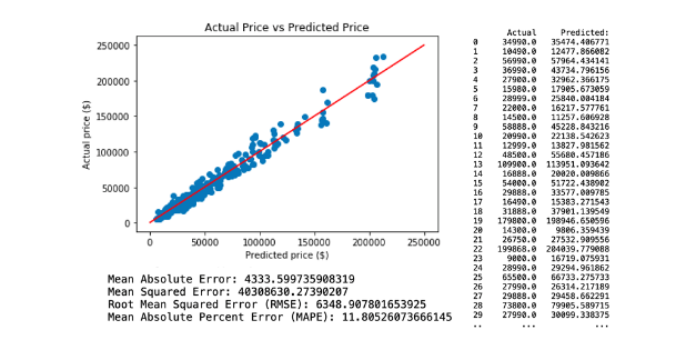
The attributes applied for regression model 2. comprises Age, KM, Engine Size, Gears, Weight and Fuel Cost. This model resulted in a Root Mean Square Error (RMSE) of 19334.10. The regression and model evaluation result is shown below.

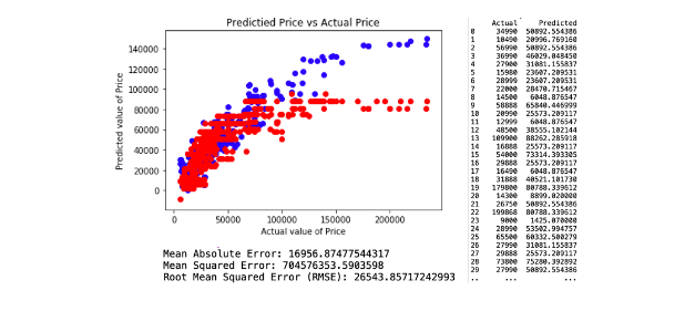
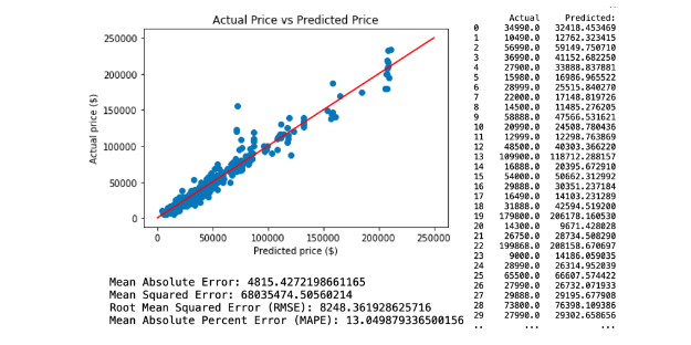
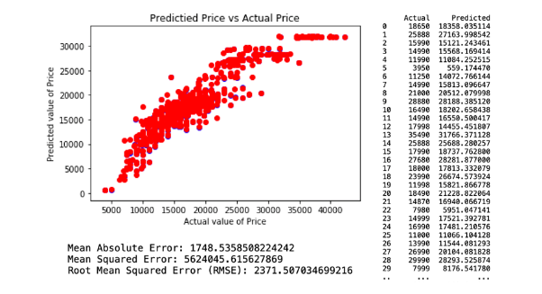
c. Regression Model 3.

The attributes applied for regression model 3. comprises Age, KM and Weight. This model resulted in a Root Mean Square Error (RMSE) of 26543.85. The regression and model evaluation result is shown below.

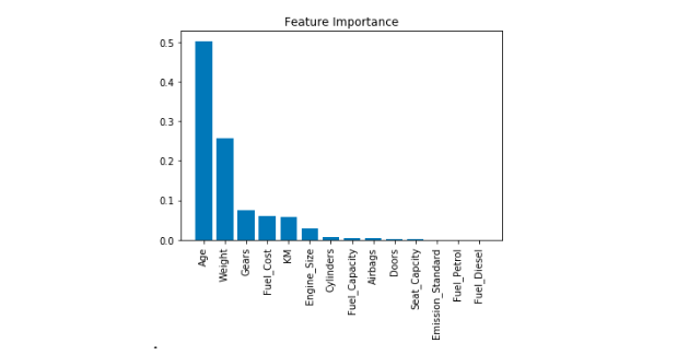
2. Random Forest Regression

As can be seen from the graph, feature Importance for Luxury shows that Age and Weight are the highest features contributing to the final price followed by Gears, Fuel Cost and KM.

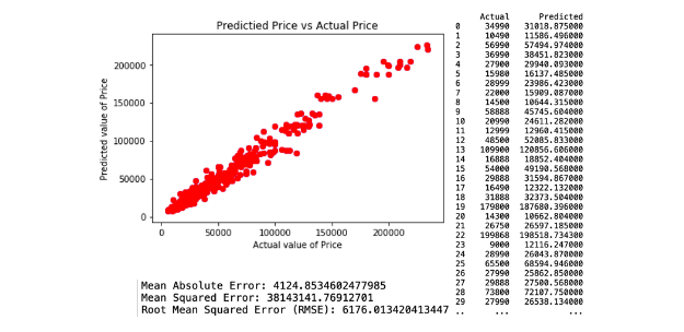
a. Regression Model 1.

The first decision tree predictive model is created by applying all selected variables and resulted with RMSE of 6176.01. The regression and model evaluation result is shown below.

b. Regression Model 2.

The second decision tree predictive model is created by applying features that have an importance of more than 0.01. There are 6 selected variables of feature importances, which comprises of Age, KM, Engine Size, Gears, Weight and Fuel Cost. This resulted with RMSE of 6216.75. The regression and model evaluation result is shown below.

c. Regression Model 3.

The third neural network predictive model is created by applying selected variables from random tree regression model 3, which comprises Age, KM and Weight. This resulted with RMSE of 7941.43. The regression and model evaluation result is shown below.

3. Neural Network Regression

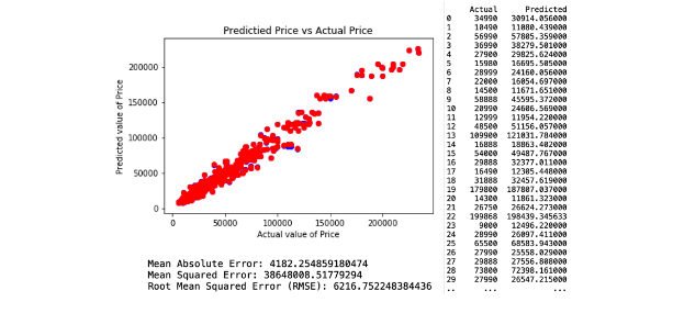
a. Regression Model 1.

The first neural network predictive model is created by applying all selected variables. This resulted with RMSE of 6302.07. The regression and model evaluation result is shown below.

b. Regression Model 2.

The second neural network predictive model is created by applying selected variables from random tree regression model 2, which comprises Age, KM, Engine Size, Gears, Weight and Fuel Cost. This resulted with RMSE of 6348.90. The regression and model evaluation result is shown below.

c. Regression Model 3.

The third neural network predictive model is created by applying selected variables from random tree regression model 3, which comprises Age, KM and Weight. This resulted with RMSE of 8248.36. The regression and model evaluation result is shown below.

4. Model Comparison

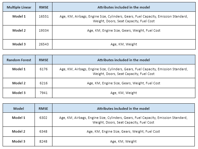
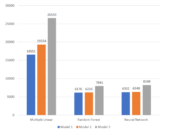
The graph above summarizes the results of three regression techniques (multiple linear/random decision tree/neural network) to predict car sales price from Luxury dataset. The accuracy of the predictive models are compared based on their RMSE. In terms of efficiency, the random forest and neural network regression technique is much more efficient compared to the multiple linear regression. From all of the above predictive models, the random forest regression technique model 1. has the lowest RMSE of 6176, however both Random Forest and Neural Network predictive models perform almost identical. Random forest shows that Age, KM and Weight are the most important features in Luxury cars. Moreover, it appears that the results from random forest slightly outperformed the results from neural network models. Consequently, both Random Forest and Neural Network models appears to be more suitable predictive modelling for the Luxury car dataset from Carsales.

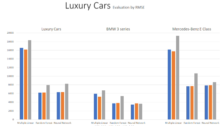
The graph above illustrates all results of three regression techniques (multiple linear/random decision tree/neural network) to predict car sales price from Luxury Cars, BMW 3 series and Mercedes-Benz E Class. The accuracy of the predictive models are compared based on their RMSE. When we go deep into more specific car makes like BMW 3 series or Mercedes-Benz E class in Luxury Cars, they performs slightly difference compared to Luxury Cars dataset. Although all three dataset shows that random forest and neural network outperformed from all results from multiple linear, by providing a more lower of RMSE. Neural Network regression model 1 from BMW 3 series appears a little lower RMSE than Random Forest models. However, the random forest technique is slightly better efficient compared to the neural network regression in Mercedes-Benz E Class. Overall, the random forest and neural network technique model appears to be more suitable predictive modelling for all Luxury Cars, BMW 3 series and Mercedes-Benz E Class cars from Carsales.

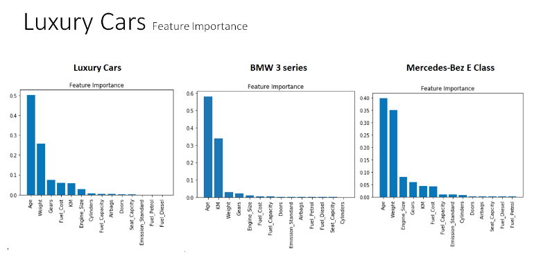
The charts above shows all the feature importance using Random Forest regression, compared with Luxury, BMW 3 series and Mercedes-benz E Class car makes. The luxury cars dataset shows that Age and Weight are the most influential features to predict car sales price, come along with Gears, Fuel Cost and KM. However, BMW 3 series dataset appears that Age and KM are the significant factors contributing to the price more than Weight. It appears that Weight and Gears features are much lower importance compared to luxury cars and Mercedes-Benz E Class. It also shows that the most substantial features of used cars are Age and Weight in Mercedes-Benz E Class, which is similar to Luxury Cars data. However, Engine Size and Gears are the next substantial features for the price in Mercedes-Benz E Class, compared to Gears, Fuel Cost and KM in Luxury Cars. As you can see, KM is not an identical features for Luxury Cars and Mercedes-Benz E Class compared to BMW 3 series. Overall, all Luxury Cars, BMW 3 series and Mercedes-Benz E Class have different car factors vital to the used car prices.

C. Economy Cars

The dataset comprises of 21 attributes related to 3992 Economy Cars which contains 3 car makes (2030 samples from Toyota Corolla, 1016 from Mazda 3 and 946 from Hyundai i30 where extracted from Carsales website).

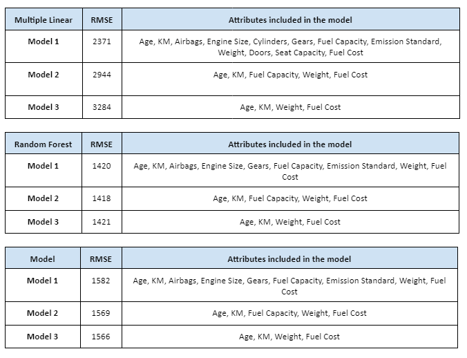
1. Multiple Linear Regression

a. Regression Model 1.

The first regression model technique predictive model has included all of the attributes in the selected variables identified previously section. This model resulted in a Root Mean Square Error (RMSE) of 2371.50. The regression and model evaluation result is shown below.

b. Regression Model 2

The attributes applied for regression model 2. comprises Age, KM, Fuel Capacity, Weight and Fuel Cost. This model resulted in a Root Mean Square Error (RMSE) of 2944.35. The regression and model evaluation result is shown below.

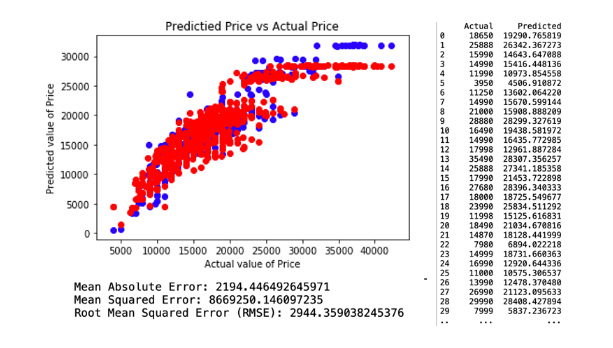
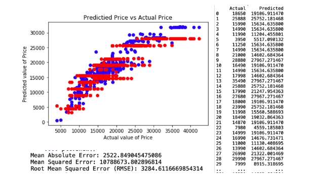
c. Regression Model 3

The attributes applied for regression model 3. comprises Age, KM, Weight and Fuel Cost. This model resulted in a Root Mean Square Error (RMSE) of 3284.61. The regression and model evaluation result is shown below.

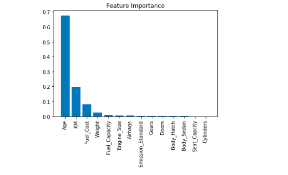
2. Random Forest Regression

As can be seen from the graph, feature Importance for Economy Cars shows that Age and KM are the highest features contributing to the final price followed by Fuel Cost.

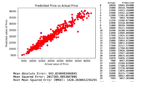
a. Regression Model 1.

The first decision tree predictive model is created by applying all selected variables and resulted with RMSE of 1420.28. The regression and model evaluation result is shown below.

b. Regression Model 2

The second decision tree predictive model is created by applying features that have an importance of more than 0.01. There are 9 selected variables of feature importances, which comprises of Age, KM, Fuel Capacity, Weight, Fuel Cost. This resulted with RMSE of 1418.63. The regression and model evaluation result is shown below.

c. Regression Model 3

The third decision tree predictive model is created by applying features that have an importance of more than 0.1. There are 4 selected variables of feature importances, which comprises of Age, KM, Fuel Cost and Weight. This resulted with RMSE of 1421.67. The regression and model evaluation result is shown below.

3. Neural Network Regression

a. Regression Model 1.

The first neural network predictive model is created by applying all selected variables. This resulted with RMSE of 1582.81. The regression and model evaluation result is shown below.

b. Regression Model 2

The second neural network predictive model is created by applying selected variables from random tree regression model 2, which comprises Age, KM, Fuel Capacity, Weight and Fuel Cost. This resulted with RMSE of 1569.02. The regression and model evaluation result is shown below.

c. Regression Model 3

The third neural network predictive model is created by applying selected variables from random tree regression model 3, which comprises Age, KM, Weight and Fuel Cost. The regression and model evaluation result is shown below.

4. Model Comparison

The graph above summarizes the results of three regression techniques (multiple linear/random decision tree/neural network) to predict car sales price from Economy Cars dataset. The accuracy of the predictive models are compared based on their RMSE. In terms of efficiency, the random forest and neural network regression technique is much more efficient compared to the multiple linear regression. In addition, it appears that the results from random forest a little outperformed the results from neural network models, by providing a more lower of RMSE. From all of the above predictive models, the random forest regression technique model 2. has the lowest RMSE of 1418. Moreover, random forest shows that Age, KM and Fuel Cost are the most important features. Overall, the random forest predictive models appears to be more suitable predictive modelling for the Economy Cars from Carsales.

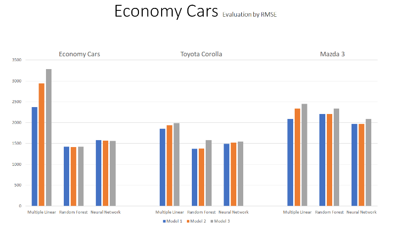
The graph above describes all results of three regression techniques (multiple linear/random decision tree/neural network) to predict car sales price from Economy Cars, Toyota Corolla and Mazda 3. The accuracy of the predictive models are compared based on their RMSE. When we go deep into more specific car makes like Toyota Corolla or Mazda 3 in Economy Cars, they perform slightly different compared to Economy Cars dataset. Although all three dataset shows that random forest and neural network outperformed from all results from multiple linear, by providing a more lower of RMSE. Random Forest in Economy Cars and Toyota Corolla appears lower RMSE than Neural Network models. However, in Mazda, the Neural Network technique performs better efficient compared to the random forest regression. Overall, the random forest model appears to be more suitable predictive modelling for Economy Cars, Toyota Corolla, on the other hand, neural network models is more suitable for Mazda 3.

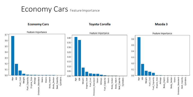
The charts above describes all the feature importance using Random Forest regression, compared with Economy Cars, Toyota Corolla and Mazda 3 car makes. All three feature importance shows that the most substantial features contributing to the price are Age and KM. However, KM is more important features in Toyota Corolla (more than 0.2), compared to less than 0.2 in Economy Cars and Mazda 3. It appears that the most substantial features of used cars are Age, KM and Fuel Cost in Economy Cars. On the other hand, Toyota Corolla shows feature importance of Age, KM and Weight. Moreover, Age, KM, Weight and Fuel Cost are substantial features for the price in Mazda 3. Overall, all Economy Cars, Toyota Corolla and Mazda 3 have in common importance factors in Age and KM, but have different other car important factors contributing to the final price of used cars.

Part 6 Conclusion

To summarize, it can be concluded that the performance of predictive modelling techniques and important features depends on car categories and makes. Accordingly, a good practice is to compare the performance of different predictive models to find the best one for the particular case in category and make. There are two approaches with Random Forest and Neural Network, which have the most potential to produce optimal regression models. As can see from the data, most of the used car data are predominantly non-linear relationships in Carsales, so multiple linear is always not suitable because it can only capture linear relationships. Both random forest and neural networks, have the ability to model linear as well as complex nonlinear relationships. An important finding in this research is that no single algorithm works best across all possible scenarios. The performance of predictive models varies depending on the application and dimensionality of the dataset depends on the car categories and individual makes. Moreover, important features contributing to the car prices give a variety according to each car category and makes, for example, feature importance of Luxury Sports - KM and Engine Size against feature importance of Ferrari - Age and KM. Following can be summarized the findings from this research.

• Use of real data and modelling categories shows that the same model is not effective for all cars.

• Predictive modelling technique performance depends on the car category and make.

• Important features change according to each car category and make.

However, there is often not enough time to test and optimize every algorithm in order to its quality in a specific criteria such as robustness, cost and time expenditure. For example, a model that performs very well with the data used to create it does not necessarily perform equally well with new data. There may contain some errors and outliers in which at any time and often by chances changes in the relationships can occur. The costs and time required for the build predictive models also can be important criteria to calculated and tested. We can expect to measure those criteria in further research.